1. Librería RCommander y técnicas de análisis estadístico.

Contenidos

• ¿Qué es RCommander?
• Aspecto de la interfaz de R Commander
• Directorio de trabajo, scripts, resultados y workspace de R
• Distribuciones de probabilidad
• Importar conjuntos de datos (I)
  
• Análisis estadísticos
• Tablas de contingencia y tests de proporciones
• Nivel avanzado: Gráficos más complejos
• Otros gráficos en Rcmdr
• Tests de medias y de varianzas
• Esquema de aplicación de test de comparación de medias
• Esquema de aplicación de test de comparación de medias (medidas repetidas)
• Tests no paramétricos
• Modelos estadísticos: ANOVA
• Esquema de aplicación de test ANOVA
• Modelos estadísticos: ANOVA de varios factores
• Modelos estadísticos: Regresión
• Análisis de modelos
• Nivel avanzado: Intervalos de confianza y predicción de la regresión
• Modelos estadísticos: Clustering

¿Qué es RCommander?

• Es una interfaz gráfica de usuario (GUI)

• Facilita el manejo de R y permite generar instrucciones de R

• Incluye la posibilidad de realizar distintos tipos de análisis (análisis exploratorio, distribuciones de probabilidad, inferencia paramétrica y no paramétrica, análisis de la varianza de uno o varios factores,....)

• Es una librería que no está incluida en la instalación base de R

install.packages('Rcmdr') 

• Una vez instalada, sólo hace falta iniciarla en cada nueva sessión de R de la siguiente forma

library(Rcmdr) # tarda un poco puesto que conviene instalar las librerías adicionales que solicita

• Si se cierra R-Commander (Rcmdr) pero no la sesión de R, se vuelve a cargar

Commander() 

Aspecto de la interfaz de R Commander

• La interfaz de R commander tiene varias partes principales
• En la parte superior se presentan una serie de opciones de menú (Fichero, Editar, ...)
• A continuación, hay dos ventanas principales:
• R Script, donde aparecen todas las instrucciones que se generarán cuando seleccionemos opciones del menú superior.
• Salida, donde se presenta en formato texto el resultado de la ejecución de las diferentes opciones del menú

Directorio de trabajo, scripts, resultados y workspace de R

• El menú 'Fichero' sirve para gestionar las instrucciones a ejecutar, los objetos creados en R, los resultados generados, etc... pero NO permite cargar conjuntos de datos para el análisis.
• El directorio de trabajo representa el directorio local donde queremos trabajar (donde estan los archivos a cargar, donde queremos guardar los scripts, ...)
• Las instrucciones de la ventan R Script (cargarlas o guardarlas)
• Los resultados de la ventana Salida (guardar)
• El entorno de trabajo (workspace) con todas las variables que tenemos creadas

• En principio, las opciones más importantes de este menú sería 'Cambiar directorio de trabajo' (al comenzar a utilizar Rcmdr) y 'Guardar las instrucciones' (al finalizar nuestra sesión de Rcmdr).

• En cualquier caso, al cerrar Rcmdr también nos preguntará si queremos guardar el script y el espacio de trabajo.

Distribuciones de probabilidad

• El menú 'Distribuciones' dispone de diversas funciones para estudiar diferentes tipos de distribuciones. En particular
• Se pueden obtener los cuantiles teóricos para una distribución (por ejemplo, para hallar cual es el valor crítico z_α/2 de una normal)
• Se pueden obtener las probabilidades Pr(Z < z)
• Representar las funciones de densidad y de probabilidad
• Generar una muestra simulada para una distribución determinada

Ejercicio 1

• Cuantiles teóricos: Obtener un vector y con los cuantiles 25%,50%,75%,100% de la normal de media 0 y sd. 1.

• Obtener una muestra de 100 valores aleatorios de una uniforme entre 0 y 1.

• Cuantiles muestrales: Obtener un vector x con los cuantiles 25%,50%,75%,100% de la muestra (se utiliza la función quantile()).

• Hacer un plot(x,y); abline(0,1)

Importar conjuntos de datos (I)

• El menú Datos nos permite importar conjuntos de datos desde varios formatos (txt, SPSS, Excel, ...). Vamos a cargar el conjunto de datos 'ddt.txt':
• group: Grupo de observaciones (mediciones en dos temporadas)
• location: Código del lugar de captura (de 1 a 3)
• location_name: Nombre del lugar (afluente, medio, desembocadura)
• species: Código de especie (de 1 a 2)
• species_name: Nombre de la especie del pez (buffalo, catfish)
• length: Longitud del pez(en cm.)
• weight: Peso pez (en grs.)
• DDT_conc: Concentración de DDT (% de peso) medida

• Se puede descargar el archivo en local y luego importarlo pero también existe la posbilidad de leer directamente desde internet

  * http://cpgonzal.github.io/cursoIntroR/ddt.txt

  * http://dl.dropboxusercontent.com/u/17677514/ddt.txt

Importar conjuntos de datos (II)

• La opción 'Conjunto de datos activo' permite:
• Filtrar observaciones (filas) del conjunto de datos
• Ver nombres de las variables (columnas) del conjunto de datos
• Guardar el conjunto de datos (en formato R) o exportar a formato texto plano

• La opción 'Modificar variables del conjunto de datos activo' permite:
• Renombrar las variables
• Calcular nuevas variables
• Tipificar o estandarizar las variables
• Reordenar niveles de un factor

Análisis estadísticos

• El menú Estadísticos nos permite realizar diversos análisis estadísticos.

• En la opción 'Resúmenes' podemos:
• Obtener resúmenes estadísticos de las variables conjunto de datos. Estos resúmenes se pueden hacer por grupos de una variable factor.
• Hallar correlaciones entre variables (Pearson, Spearman, parcial).
• Realizar test de correlaciones significativas y de normalidad de las variables.

• La opción 'Gráficas' nos permite complementar los análisis mediante
• Gráficos histograma para estudiar la distribución de los datos
• Diagramas de caja para analizar la varianza de las variables

Tablas de contingencia y tests de proporciones

• En la opción 'Tablas de contingencia' podemos generar tablas de contingencia (de doble o múltiple entrada) para analizar relaciones entre dos o más variables factor.
• REQUISITOS: Es preciso tener, al menos, 2 variables factor para generar este tipo de tablas.

• A partir de las tablas de doble entrada se pueden realizar tests de independencia de la chi-cuadrado

• En la opción 'Proporciones' podemos realizar pruebas sobre la proporción de éxitos (o de un grupo determinado) en una población
• REQUISITOS: Es preciso tener 1 variable factor con 2 niveles para realizar este test.

Ejercicio 2

• Realizar un resumen descriptivo de 'DDT_conc' para cada uno de los 2 grupos de observaciones.

• Realizar un test para comparar si la proporción de observaciones en el grupo 1 es igual a la del grupo 2

• Realizar una tabla de contingencia para comparar los 2 grupos de observaciones con las 3 especies de peces.

• PISTA: La variable 'group' ha sido cargada en R como variable numérica y debería ser un factor.

• Realizar un histograma comparativo del 'DDT_conc' del grupo 1 con el grupo 2

Nivel avanzado: Gráficos más complejos

• Se puede hacer un gráfico histograma combinado con diagrama de cajas y añadir una curva de densidad normal

#require(devtools)
#ddt<-read.table("ddt.txt",header=TRUE,sep="",dec=".")
devtools::source_gist("1e7ee71e79346ffdd5a5",filename = "plotHistBox.R")
plotHistBox(ddt$length)

Nivel avanzado: Gráficos más complejos

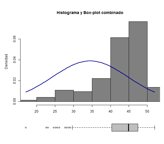
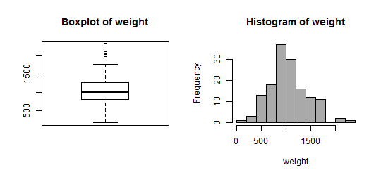
• Los gráficos histogramas también se pueden combinar

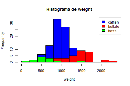
h1<-hist(ddt$weight, col="grey60",main="Histograma de weight",xlab="weight")

par(mfrow=c(1,1) )
with(ddt, hist(weight[species==1], breaks=h1$breaks, col="blue",main="Histograma de weight",xlab="weight" ))
with(ddt, hist(weight[species==2], breaks=h1$breaks, col="red",add=TRUE ))
with(ddt, hist(weight[species==3], breaks=h1$breaks, col="green",add=TRUE ))

legend( "topright", sort(levels(ddt$species_name),decreasing = TRUE) , fill=c("blue", "red","green") )

Otros gráficos en Rcmdr

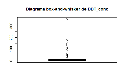
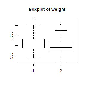
• Los gráficos de cajas y bigotes

boxplot( ddt$DDT_conc, main="Diagrama box-and-whisker de DDT_conc",col="gray")

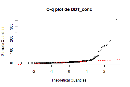
• Los gráficos de comparación de cuantiles (qq-plot)

qqnorm( ddt$DDT_conc, main="Q-q plot de DDT_conc")
qqline(ddt$DDT_conc, col="red", lty="dashed")

Otros gráficos en Rcmdr

• Los gráficos 'Diagrama de dispersión' permiten representar 2 variables y añadir la información de un grupo.

require(car)
scatterplot(length~weight | group, regLine=TRUE, smooth=FALSE, 
  boxplots=FALSE, by.groups=TRUE, reset.par=FALSE, 
  data=ddt)

Otros gráficos en Rcmdr

• Otro gráfico de 2 variables es 'Gráfica XY'

require(lattice)
xyplot(length~weight , groups=group, type="p", pch=16,
       auto.key=list(border=TRUE),data=ddt)

Otros gráficos en Rcmdr

• Los gráficos 'Matriz de diagrama de dispersión' permiten visualizar múltiples variables

scatterplotMatrix(~DDT_conc+length+weight, regLine=TRUE, smooth=FALSE, 
  diagonal = TRUE, data=ddt)

Otros gráficos en Rcmdr

• Los 'Gráficos de medias' son muy útiles en ANOVAs

require(Rcmdr)
plotMeans(ddt$DDT_conc, ddt$species_name, error.bars="conf.int", level=0.95)

Tests de medias y de varianzas

• En la opción 'Medias' podemos realizar pruebas sobre la media estadística de una o más poblaciones.
• El test “Test t para una muestra” corresponde a la prueba clásica sobre la media de una población cuando la varianza es desconocida.
• Los “Test t para muestras independientes” y “Test t para datos relacionados” permiten comparar, dadas dos muestras (o dos grupos), las medias de sus respectivas poblaciones.
• REQUISITOS: Para realizar el test de muestras independientes, Rcmdr necesita una variable factor con dos niveles para diferenciar cada muestra.
• Los tests "ANOVA" nos permiten comparar medias para un mayor número de niveles o grupos (2 ó más).

• En la opción 'Varianzas' se puede analizar la varianza estadística de una o más poblaciones
• El test F-ratio contrasta, dadas dos muestras, el cociente de varianzas de sus respectivas poblaciones.
• REQUISITOS: De nuevo, en Rcmdr es preciso una variable factor con dos niveles para diferenciar cada muestra.
• Otros tests que permiten comparar la igualdad de varianzas entre mayor número de niveles son el test de Bartlett y el de Levene.

Esquema de aplicación de test de comparación de medias

Esquema de aplicación de test de comparación de medias (medidas repetidas)

Ejercicio 3

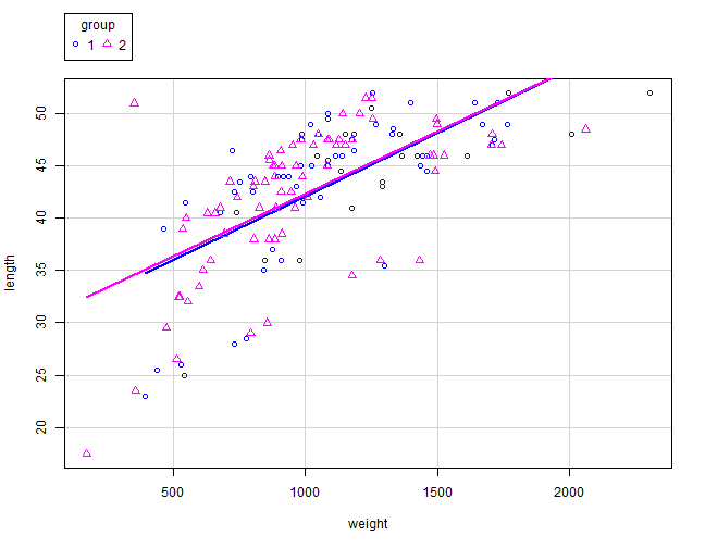
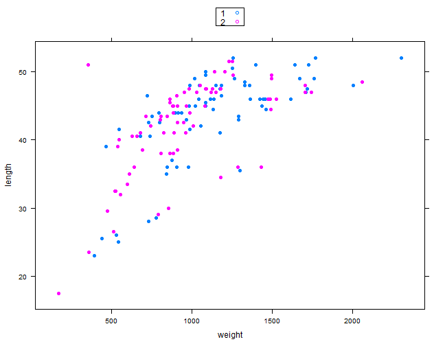
Comparar el peso de los peces del grupo 1 con el peso de los del grupo 2.

• 1º PASO: ¿Se asume normalidad de la variable peso?

shapiro.test(ddt$weight)

## 
##  Shapiro-Wilk normality test
## 
## data:  ddt$weight
## W = 0.9825, p-value = 0.06299

Si hay dudas en la normalidad, el t-test no se puede aplicar y hay que acudir a alternativas no paramétricas.

Ejercicio 4

Comparar el peso de los peces del grupo 1 con el peso de los del grupo 2.

• 2º PASO: ¿Se asume igualdad de varianzas de peso entre los grupos?
  

bartlett.test(weight ~ group, data=ddt)

## 
##  Bartlett test of homogeneity of variances
## 
## data:  weight by group
## Bartlett's K-squared = 0.13287, df = 1, p-value = 0.7155

Si las varianzas entre grupos son iguales, se debe especificar en opciones del t-test (aprox. Welch).

Tests no paramétricos

• En la opción 'Tests no paramétricos' se pueden realizar distintas pruebas de estadísticas cuando no se verifican ciertas hipótesis.
• El “test de Wilcoxon” es equivalente al t-test para muestras independientes cuando no se puede asumir normalidad en los datos.
• El “test de Kruskal-Wallis” y el “test de Friedman” son tests basados en el rango muestral de las observaciones (equivalentes al ANOVA cuando no se puede asumir normalidad).

• EJEMPLO: Comparar 'DDT_conc' de los peces del grupo 1 con los del grupo 2.

Modelos estadísticos: ANOVA

• La opción 'Medias' permite realizar el análisis de varianza de uno o varios factores para comparar las medias de grupos (similar al t-test pero con 2 o más niveles en las variables factor).

• La opción 'Tests no paramétricos', con los “test de Kruskal-Wallis” y el “test de Friedman”, son pruebas no paramétricas alternativas al ANOVA.

• Junto a la 'Gráfica de las medias' permite llevar a cabo un análisis comparativo de los efectos de los factores y sus interacciones en un modelo.

Esquema de aplicación de test ANOVA

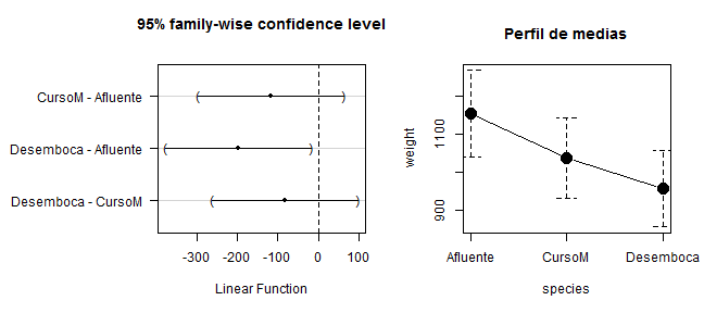
Ejercicio 5

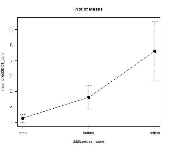
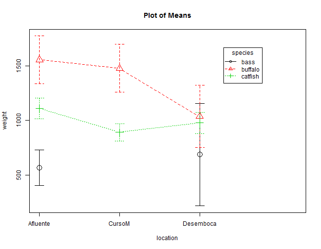
• EJEMPLO: Analizar las diferencias en el peso de los peces entre las diferentes localizaciones.

• 1º PASO: ¿Hay diferencias entre todos los niveles (especies)?

# Comprobamos si la varianza es constante
bartlett.test(weight ~ location_name, data=ddt)

## 
##  Bartlett test of homogeneity of variances
## 
## data:  weight by location_name
## Bartlett's K-squared = 0.78832, df = 2, p-value = 0.6742

# En caso de homoc. podemos hacer anova
anova.mod1 <- aov(weight ~ location_name, data=ddt)
summary(anova.mod1)

##                Df   Sum Sq Mean Sq F value Pr(>F)  
## location_name   2   942700  471350   3.438 0.0349 *
## Residuals     141 19332838  137112                 
## ---
## Signif. codes:  0 '***' 0.001 '**' 0.01 '*' 0.05 '.' 0.1 ' ' 1

# Si no se asume var. cte. o no hay normalidad, recurrimos al test K.-W.
kruskal.test(weight ~ location_name, data=ddt)

## 
##  Kruskal-Wallis rank sum test
## 
## data:  weight by location_name
## Kruskal-Wallis chi-squared = 6.13, df = 2, p-value = 0.04665

Ejercicio 6

• EJEMPLO: Analizar las diferencias en el peso de los peces entre las diferentes localizaciones.

• 2º PASO: ¿Cómo son las diferencias 2 a 2? (sólo si hay más de 2 niveles en el factor)

anova.mod1 <- aov(weight ~ location_name, data=ddt)
summary(glht(anova.mod1, linfct = mcp(location_name = "Tukey"))) # pairwise tests

Modelos estadísticos: ANOVA de varios factores

• En el ANOVA de múltiples factores es posible analizar no sólo los efectos simples sino también las interacciones.

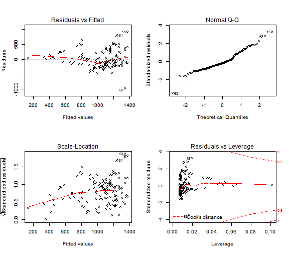
Modelos estadísticos: Regresión

• La opción 'Ajuste de modelos' dispone de múltiples posibilidades para la creación de modelos estadísticos.

• Además, en la opción 'Modelos' se pueden llevar a cabo muchos análisis habituales en el estudio de los mismos.

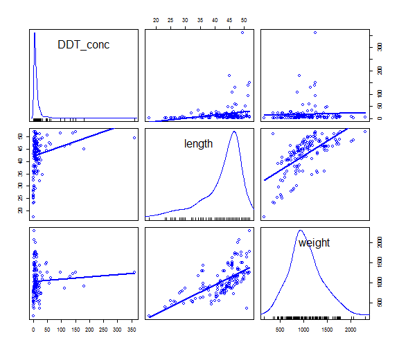
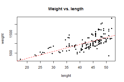
• En particular, veamos como determinar un modelo de regresión para estudiar la relación entre la longitud y el peso de los peces.

regmod.1 <- lm(weight~length, data=ddt)
summary(regmod.1)

## 
## Call:
## lm(formula = weight ~ length, data = ddt)
## 
## Residuals:
##     Min      1Q  Median      3Q     Max 
## -989.96 -189.45  -49.51  193.68  923.22 
## 
## Coefficients:
##             Estimate Std. Error t value Pr(>|t|)    
## (Intercept) -483.672    150.497  -3.214  0.00162 ** 
## length        35.816      3.471  10.319  < 2e-16 ***
## ---
## Signif. codes:  0 '***' 0.001 '**' 0.01 '*' 0.05 '.' 0.1 ' ' 1
## 
## Residual standard error: 285.7 on 142 degrees of freedom
## Multiple R-squared:  0.4285, Adjusted R-squared:  0.4245 
## F-statistic: 106.5 on 1 and 142 DF,  p-value: < 2.2e-16

Análisis de modelos

• Podemos obtener la correlación de las variables de interés en 'Estadísticos->Resúmenes'.

cor(ddt[,c("length","weight")], use="complete")

##           length    weight
## length 1.0000000 0.6546113
## weight 0.6546113 1.0000000

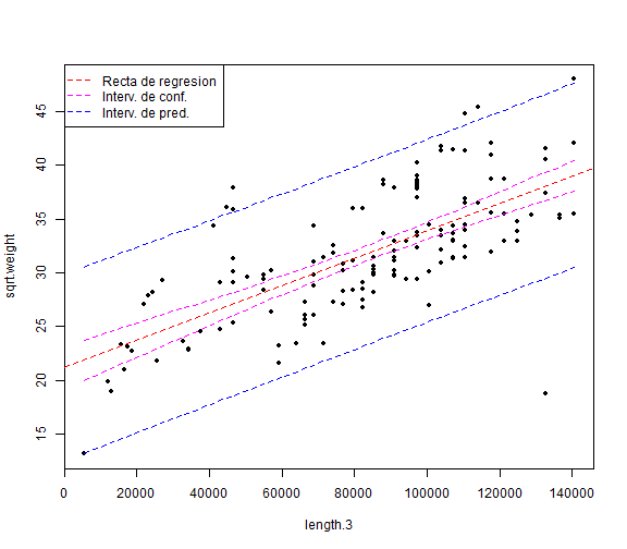
• La representación gráfica de un modelo simple es posible en 'Gráficas->Diagrama de dispersión' seleccionando la opción de mínimos cuadrados. Pero se puede hacer también con plot() y abline()

plot(ddt$length, ddt$weight, main="Weight vs. length", xlab="lenght", ylab="weight",
     pch=20)
abline(regmod.1,col="red",lty="dashed")

Análisis de modelos

• Con el menú 'Modelos->Gráficas->Gráficas básicas de diagnóstico' se pueden obtener una serie de gráficos útiles para el diagnóstico de las hipótesis habituales (homocedasticidad, normalidad, observaciones atípicas)

par(mfrow=c(2,2))
plot(regmod.1)

Ejercicio 7

• Parece que el modelo weight = β₀ + β₁length + ϵ presenta problemas.

• SUGERENCIA: Transformar variables length ⇒ length³ y weight ⇒ sqrt(weight) y volver a hacer el ajuste.

• En Rcmdr se encuentran disponibles otros análisis útiles en regresión (Breusch-Pagan para la homocedasticidad, Durbin-Watson para la independencia).

Nivel avanzado: Intervalos de confianza y predicción de la regresión

• Para los modelos lineales simples, se pueden representar los intervalos de confianza y predición de la recta

ddt$length.3 <- ddt$length^3
ddt$sqrt.weight <- sqrt(ddt$weight)
source_gist("f9b06d411675c1702ccc",filename="plotConf.R")
plotConf(sqrt.weight~length.3, ddt)

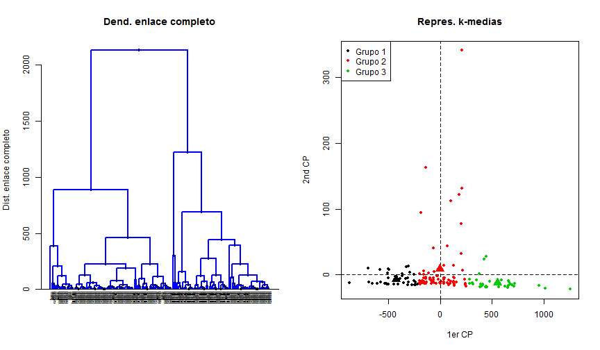
Modelos estadísticos: Clustering

• La opción 'Análisis dimensional->Análisis de agrupación' permite aplicar técnicas de cluster.

require(devtools)
source_gist("a4b2ed204d01bc12d952",filename="plotCluster.R")
par(mfrow=c(1,2))
par(mfrow=c(1,2))
plotCluster(1,ddt[,c("length","weight","DDT_conc")],ddt$species_name)
plotCluster(2,ddt[,c("length","weight","DDT_conc")],ddt$species_name)